%run src/init_notebooks.py
check_notebook()
hide_toggle()
Umbrella sampling
Questions this tutorial will address
How can I get insight faster than with plain molecular dynamics?
What problems can umbrella sampling help with?
How should I design and set up umbrella sampling simulations?
Metadata
Version: 2021
Contributions: Dr Mark Abraham, Dr Christian Blau
Supported by: ENCCS (https://enccs.se/), BioExcel (https://bioexcel.eu/)
Target audience
The content of this tutorial suits experienced users of GROMACS. Such users should be familiar with basic theory behind MD simulations, along with setting them up and running them in GROMACS.
Prerequisites
GROMACS 2021 or later (other versions will likely work, but might look a bit different)
Optional
a molecular viewer, e.g. VMD
a plotting tool, e.g. xmgrace
What is umbrella sampling?
Many modelling problems require sampling transitions between coarse states. In principle, molecular dynamics simulations will eventually undertake those transitions often enough that insight into paths, barrier sizes, and rates can be gained. But that is extremely inefficient. We would often like to be able to guide or pull the sampling to where we need it.
Example: membrane permeation
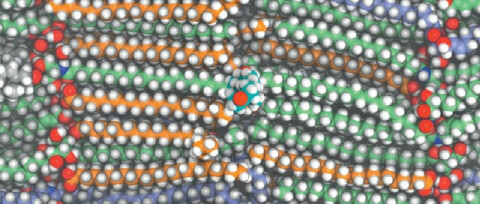 The permeability of
skin to drugs can be estimated by pulling a drug (in the center) across
the bilayers that remain after skin cells dry.
The permeability of
skin to drugs can be estimated by pulling a drug (in the center) across
the bilayers that remain after skin cells dry.
Example: host-guest binding
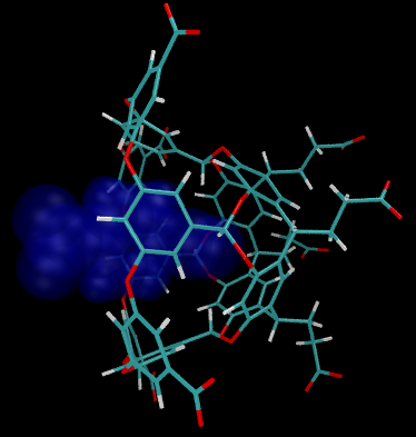 Host-guest systems model ligands
binding to biomacromolecules. The free-energy of binding can be
estimated by pulling the blue guest away from the wireframe host.
Host-guest systems model ligands
binding to biomacromolecules. The free-energy of binding can be
estimated by pulling the blue guest away from the wireframe host.
Pathways for pulling
Given an initial guess at a pathway, it is much more efficient to bias the sampling to places that lie on that pathway. The system is allowed to explore the equilibrium state described by the normal molecular potential plus the bias. The observed frequencies of configurations can then be re-weighted to remove the effect of the bias. The resulting unbiased samples can be used to get insight into e.g. changes in free energy along the pathway.
In the above examples, simple paths for pulling would lie in the horizontal direction, between centers of mass of different groups. Sometimes simple paths do not exist and need to be composed piece-wise.
Model system for this tutorial
In this tutorial, we will use a simple system that needs only moderate resources to sample. Nevertheless, it captures a lot of the essential complexity that characterizes real problems. We will use umbrella sampling, also known as pulling, to examine the free-energy profile of bringing two pyrimidine molecules together in an aqueous solution.
 A single molecule of pyrimidine
We want to estimate the free energy of binding of two such molecules, and make any observations that we can about the pathway of binding. For the path, or reaction coordinate we will choose the vector that joins the center of mass of two pyrimidine molecules. We will run simulations along that pathway to understand the conformations that are adopted there. To locate the free-energy minimum of any bound conformation we will need to bring them quite close together (ie. < 1 nm) and also quite far apart.
Quiz
How far apart do we need to take the molecules in order to estimate the free energy of binding?
Infinitely far
1 nm
5 nm
It depends
Sampling a reaction coordinate
Ideally, we would run just one simulation in the bound state and one in the free state. They would both happen to visit similar conformations, and we could compute the free energy of the transition between bound and free states directly.
This is possible to do, but rarely efficient. Instead we run many simulations, each at different positions along the reaction coordinate. We try to choose the points close enough together that some of the sampling at each point will be of configurations that are also close to adjacent points along the path. If successful, this means that we can estimate the free-energy difference of going from one point to another. Doing that pairwise estimation along the whole pathway means we can estimate the free-energy difference of the whole pathway. Remember that free energy differences are independent of the path taken between the states!
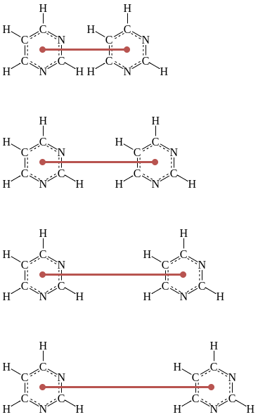 A series of displacements (shown in dark red)
along a reaction coordinate are chosen to create a series of simulations
whose configuration ensembles overlap those of adjacent simulations.
A series of displacements (shown in dark red)
along a reaction coordinate are chosen to create a series of simulations
whose configuration ensembles overlap those of adjacent simulations.
Quiz
What would happen if the displacements are chosen too far apart?
The overall computation would be more efficient
The overall computation would be less efficient
The result would be more likely to be correct
The result would be less likely to be correct
The biasing potential
Once the reaction coordinate and sampling locations are chosen, a very common choice of biasing potential is harmonic in the displacement along that coordinate. The shape of an harmonic potential is like an upside-down umbrella, which is how one name for this enhanced-sampling method came about!
One simulation is run at each single location along the reaction coordinate, and during the simulation if the system diffuses away from that location it experiences a force that tends to return it to that location. In this tutorial, we will measure the displacement between the center of mass of each molecule. During the simulation, any force on the center of mass due to the bias is distributed to the particles according to their mass.
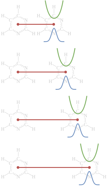 Schematic illustration of four
simulations of the same system used as part of an umbrella sampling
study. Each simulation has a different harmonic “umbrella” potential
(shown in green) that keeps it near its chosen displacement along the
reaction coordinate (shown in dark red). The umbrella displacements and
widths are carefully chosen so that the resulting configurational
ensemble (blue) for each simulation overlaps those of adjacent
simulations.
Schematic illustration of four
simulations of the same system used as part of an umbrella sampling
study. Each simulation has a different harmonic “umbrella” potential
(shown in green) that keeps it near its chosen displacement along the
reaction coordinate (shown in dark red). The umbrella displacements and
widths are carefully chosen so that the resulting configurational
ensemble (blue) for each simulation overlaps those of adjacent
simulations.
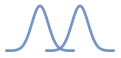 Two Gaussian distributions that
overlap are shown. How much the distributions sampled by your biased
simulations should overlap depends. Too much and you will be running
more simulations than you need to. Too little and your free-energy
profile will be inaccurate.
Two Gaussian distributions that
overlap are shown. How much the distributions sampled by your biased
simulations should overlap depends. Too much and you will be running
more simulations than you need to. Too little and your free-energy
profile will be inaccurate.
Quiz
What would happen if the harmonic potentials are too “stiff” ie. narrow in shape?
The overall computation would be more efficient
The overall computation would be less efficient
The result would be more likely to be correct
The result would be less likely to be correct
Planning for an umbrella sampling simulation
In order to do umbrella sampling, a simulation must be equilibrated at each location on the reaction coordinate, with the umbrella potential active. This can be tricky, because it is often not a simple case of “click and drag!”
Sometimes it is enough to start from either a bound or free configuration near one of the desired reaction coordinate points, and equilibrate to it. The endpoint of that equilibration might be used to start the next equilibration at an adjacent location. If the locations have been chosen well, this will work fine, because the adjacent location will sample nearby configurations that can be reached easily. However, it means that the last simulation in the series won’t start until all the other equilibrations have completed.
An alternative is to run “steered molecular dynamics” to do a non-equilbrium trajectory that is forced to move along the reaction coordinate. From that trajectory we can pick suitable configurations to start the equilibration at each location along the reaction coordinate. In GROMACS, this is called “constant-force pulling.”
Another alternative is “interactive molecular dynamics” where the user can link visualization software to a running simulation and choose where to apply forces to effect transitions. This can help to provide insight into possible reaction coordinates, as well as where to sample along them.
Discussion
All these approaches can introduce a path dependence into the configurations chosen to begin the equilibration. This might be a significant risk in a real scientific investigation. How might this be mitigated?
System preparation for this tutorial
For this tutorial, 24 systems have been prepared in advance using the first method described above. This will help us focus on the mechanics of umbrella sampling, rather than details of solvating and choosing box sizes that are common to all simulations.
However, we should now look at those mechanics!
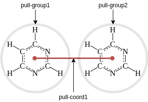
GROMACS .mdp options for pulling
Using functionality in GROMACS requires setting appropriate options in
the .mdp file. The ones we’ll use will let the simulation know that
pulling will take place, as well as describe the reaction coordinate(s)
and bias(es). GROMACS typically uses pull groups and pull geometries
to define pull coordinates (ie reaction coordinate). In the example in
this tutorial, we will use one pull group for each pyrimidine molecule.
The distances betwen the centers of mass of those groups will define the
single pull coordinate.
Pull groups and coordinates
Together, the .mdp lines for the above pulling setup are:
pull                     = yes
pull-ngroups             = 2
pull-group1-name         = pyrimidine_1
pull-group2-name         = pyrimidine_2
pull-ncoords             = 1
pull-coord1-groups       = 1 2
pull-coord1-geometry     = distance
As with other kinds of groups in GROMACS (e.g. temperature-coupling
groups), the pull groups are described by index groups in the index
file also supplied to gmx grompp (typically named index.ndx).
To use umbrella sampling, we describe that as the pull-coord-type
and choose a width for the harmonic potential pull-coord-k. In this
tutorial, the umbrella will not move so has a zero pull-coord-rate.
Finally, each system we prepare will have a fixed location chosen for
the umbrella along the reaction coordinate, here 0.834 nm.
pull-coord1-type         = umbrella
pull-coord1-k            = 5000.0
pull-coord1-rate         = 0.0
pull-coord1-init         = 0.834
These and many other .mdp options for pulling are described more
full in the
documentation.
Let us look at one of the grompp.mdp run input files:
%less sampling/run-08/grompp.mdp
Here we can see a very normal production simulation of 5 ns, using the above-mentioned pull-code options.
What range of initial reaction coordinate locations was chosen over the set of simulations? (Remember the default unit for distance is nm.)
! grep pull-coord1-init sampling/run-*/grompp.mdp
Quiz
Does that range seem suitable? * Yes * No, too many short distances * No, not enough short distances * No, too many long distances * No, not enough long distances
What differences exist between these run input files? Let’s look at two adjacent ones:
! diff sampling/run-08/grompp.mdp sampling/run-09/grompp.mdp
What is in the simulation topology?
%less sampling/run-08/topol.top
How are the index groups set up for the pull groups? Remember, the order
of atoms in the coordinate file conf.gro matches the order implied
by the [ molecules ] section above.
! head -n 10 sampling/run-08/index.ndx
Finally, let’s visualize one of the systems:
nv.show_structure_file('sampling/run-08/conf.gro')
Running gmx grompp
If you have GROMACS installed, then you can go ahead and run
gmx grompp -n in each of the sampling/run-* directories. We’ll
need the .tpr files later for the analysis, so we’ll go ahead and
use a bash loop to do that now:
%%bash
for run_directory in sampling/run-*
do
  (cd $run_directory; gmx grompp -n)
done
Running gmx mdrun
These are quite small systems, but we have a lot of them, so we won’t
try to run them together now. Even if you have a GPU, the set of them
will take 10-20 hours to run. If you did run them, then an efficient
approach on a cluster would be to use
mpiexec -np 24 gmx_mpi mdrun -multidir sampling/run*. Alternatively,
you could run them one by one with:
(for run_directory in sampling/run-*; \
 do \
   (cd $run_directory; gmx mdrun) \
 done)
In each directory, this command produces the usual .log, .xtc,
.edr, and .cpt files together with two other output files,
namely pullx.xvg and pullf.xvg. Respectively, these contain the
time series for that simulation of the distance along the reaction
coordinate, and the resulting scalar force that biases the simulation
back towards the pull-coord-init distance value.
Analysing pulling simulations with WHAM
GROMACS provides a tool called gmx wham that executes the Weighted
Histogram Analysis Method (WHAM). We will use it to analyse the biased
sampling along the reaction coordinate \(\xi\), reweight those
samples, and combine the sampling along the reaction coordinate to
return a free-energy profile along \(\xi\). That profile is also
known as a potential of mean force for historical reasons.
The free energy profile we seek, \(A(\xi)\) is related to the probability \(P(\xi)\) of finding configurations at different points on the reaction coordinate \(\xi\): \(A(\xi) = −k_\beta T \mathrm{ln} P(\xi)\) \(T\) is the temperature of our simulation, and \(k_\beta\) is Boltzmann’s constant.
However we don’t have time to wait for enough sampling to compute \(P(\xi)\) directly. Instead, we have run our series of biased simulations (indexed with \(i\) from 1 to \(N_w\)), with added umbrella potentials \(V_i(x)\). These produced a set of biased probability distributions \(P_i^\mathrm{bias}(\xi)\). We’d like to use those to estimate the unbiased free energy \(A_i(\xi)\) based on simulation \(i\) by removing the umbrella potential \(V_i(\xi)\) and the free-energy contribution from that bias, \(F_i\), after the fact: \(A_i(\xi) = −k_\beta T \mathrm{ln} P_i^\mathrm{bias}(\xi) - V_i(\xi) + F_i\) Sadly, the values of \(F_i\) depend on the bias, so there is no easy solution.
To get the most reliable estimate for \(P(\xi)\) we want to combine the information from all the biased simulations. \(P(\xi) = \Sigma_{i=1}^{N_w} w_i P_i^\mathrm{bias}(\xi)\) There exists a statistically optimal way to determine the weights \(w_i\), but going through the derivation is out of scope for this course. Please check out https://doi.org/10.1002/jcc.540130812 to see the details!
The resulting set of \(N_w + 1\) WHAM equations are \(P(\xi) = \frac{ \Sigma_{i=1}^{N_w} h_i(\xi) } { \Sigma_{j=1}^{N_w} n_j \exp ( -\beta V_j(\xi) + F_j )}\) \(\exp (F_i) = \int d\xi P(\xi) \exp(-\beta V_i(\xi) )\) where \(h_i(\xi)\) is the histogram count from simulation \(i\) observed at reaction coordinate \(\xi\), \(n_i\) is the count of total observations from simulation \(i\), and \(\beta=\frac{1}{k_\beta T}\). In practice, this requires choosing a range of \(\xi\) over which to plot a histogram, and a number of bins into which to divide the histogram.
There are multiple unknowns, namely \(P(\xi)\) and \(F_i\). In such cases, one often resorts to an iterative solution. We guess part of the solution and updating the guess until we find values that are self-consistent with all the available information. In general, that would be difficult for WHAM. However, if the simulations overlap sufficiently and have adequate sampling, we know that they should mutually agree on the value of \(P(\xi)\) in the region where they overlap. This means the iteration to find self-consistency has a decent chance to succeed.
It often works well to make a first guess of a flat free-energy profile, ie. \(F_i = 0\) for all \(i\). Thereafter, one can compute \(P(\xi)\), then update \(F_i\), etc. until the values stop changing. Then they are said to be self consistent.
Note that the above equations are simplified in several ways. Properly, one should compute the autocorrelation time of the observations and reweight them accordingly. However, in practice these times are normally the same across all \(i\) simulations. (A notable exception is phase transitions.) We have assumed that the bias potential depends only on \(\xi\), that all simulations have a common temperature, and that it is necessary to construct a histogram. Much research has gone into generalizations and improvements to umbrella simulation and WHAM protocols, and some links and further reading are found below.
Analysing our pulling simulations
The sampling along the reaction coordinate is recorded in the
pullx.xvg files created by gmx mdrun. The bias force experienced
there is computed by gmx wham based on the information in the
corresponding topol.tpr file. We provide will gmx wham with two
lists of files, respectively of pullx.xvg and topol.tpr files.
The order of the simulations within the lists does not matter, but the
pair of files for each simulation must be in matching places in the two
lists. That’s how gmx wham is able to match the observed distances
with the expected bias.
For this tutorial, those files have been provided for you, so let’s construct the lists of those files:
! ls -1 analysis/run-*/pullx.xvg > pullx.dat; cat pullx.dat; ls -1 sampling/run-*/topol.tpr > tpr.dat; cat tpr.dat
Let’s go ahead and run gmx wham with those inputs! In additional to
the terminal output, it produces two output files that we can plot.
run_command('gmx wham -it tpr.dat -ix pullx')
metadata, data = parse_xvg("profile.xvg")
plot_data(data, metadata)
By default, gmx wham will observe the range of sampled reaction
coordinate values and decide the range over which it will put samples
into histograms to compute the free energy. It reports that it
Determined boundaries to 0.289226 and 2.399760
Quiz
Is that reasonable, given the range of pull-coord-init we prepared
and checked above?
We can’t know
No
Yes
Earlier in the output, it reports
Warning, poor sampling bin 198 (z=2.38393). Check your histograms!
Warning, poor sampling bin 199 (z=2.39448). Check your histograms!
so it looks like the automatic range detection might be too ambitious. Scroll down in the output above to see the plot of the histogram, and let’s see how it looks.
The free energy required to be at each location on the reaction coordinate is estimated. It doesn’t look too bad, e.g. no sharp spike at large distances. But from the above warnings, the sampling at large distances is suspect, so let’s be more conservative. We’ll set the minimum and maximum extent of the histograms manually. It’s also convenient to set the zero of the free energy to be at large distances in this case, as that is intended to approximately model a pair of infinitely separated pyrimidine modules.
run_command('gmx wham -it tpr.dat -ix pullx -min 0.288 -max 2.35 -zprof0 2.35')
metadata, data = parse_xvg("profile.xvg")
plot_data(data, metadata)
No warning this time!
Now we can see easily that we probably haven’t chosen simulations for which the reaction coordinate far enough away to properly reach the asymptote we expect at large distances. The free energy grows slowly to a peak around 0.7 nm, reaches a trough as the pyrimidines get closer, and then spikes hard as the centers of mass get so close that van der Waals’ repulsions dominate.
Discussion - think for a minute, then write in the hackmd document
What do you think is happening around 0.5 nm? What do you think is happening when the solutes are 0.7 nm apart?
Let’s investigate by taking a look at the initial configuration taken from 0.5 nm. In a real situation, you would consider the whole trajectory, but the initial configuration is enough for this tutorial.
view = nv.show_structure_file('sampling/run-05/conf.gro')
view
Modify the line above to inspect the initial conditional also for 0.7 nm (in run-07 folder). Can you see anything to confirm your hypotheses?
Sampling overlap
A successful umbrella sampling simulation requires that the simulations
subject to the umbrellas produce configurations that overlap with those
sampled by adjacent simulations. The gmx wham tool also prints out a
convenient plot (named histo.xvg by default) that provides clues
whether that has happened. The extent of the overlap suggests whether
sufficient overlap exists. Let’s see that in action:
metadata, data = parse_xvg("histo.xvg")
plot_data(data, metadata)
It is clear that the distributions described by the simulations do overlap. If they did not overlap enough, then adding another simulation at intermediate point(s) in reaction-coordinate space would improve the results.
Was there enough sampling?
This perennial question in MD often doesn’t have a good answer. If the
converged simulation never found a relevant part of configuration space,
then just running more simulation is unlikely to help you. If we hadn’t
sampled this system enough, we’d run into problems making a histogram.
Let’s use the functionality of gmx wham to look only at the first
two nanoseconds of data, to see the kind of problems we might run into:
run_command('gmx wham -it tpr.dat -ix pullx.dat -b 0 -e 2 -bins 50')
metadata, data = parse_xvg("profile.xvg")
plot_data(data, metadata)
metadata, data = parse_xvg("histo.xvg")
plot_data(data, metadata)
Here we see that despite reasonable overlap of the limited sampling, the PMF produced has spiky artefacts. That suggests the total sampling is too low, and particularly so in the region of the artefacts (in this case, that means everywhere). If you would see this in a real simulation study, now you know what to do.
What happens if the reaction coordinate is too widely spaced?
Sometimes an initial guess for reaction-coordinate spacing is too
conservative. In such cases, the overlap between simulations is too low.
The iterative process that solves the WHAM equations will definitely
fail for lack of data in such regions. This is sometimes clearly seen in
the profile it produces. Here, we will use the bash tool called
seq to help us omit every second simulation from the sampling to
observe the kind of effect that can be seen:
%%bash
rm -f pullx.dat tpr.dat
for index in $(seq -w 0 2 23)
do
  echo "analysis/run-$index/pullx.xvg" >> pullx.dat
  echo "sampling/run-$index/topol.tpr" >> tpr.dat
done
run_command('gmx wham -it tpr.dat -ix pullx.dat')
metadata, data = parse_xvg("profile.xvg")
plot_data(data, metadata)
metadata, data = parse_xvg("histo.xvg")
plot_data(data, metadata)
Note again that warnings were seen, and the artifacts had a suggestive regularity, because the missing regions were regularly spaced. That regularity is itself an artifact of our choice to space the simulations evenly in reaction-coordinate space. If the spacing between simulations had been refined already, then you will need to consider carefully where artefacts from lack of sampling overlap might exist. Overlaying the locations of the target locations in configuration space can be helpful here.
Other possible artefacts
As with all methods that require choosing a reaction coordinate, if the choice does not capture essential features of the landscape, then the conclusions are unlikely to be correct. Exploratory studies are often needed to provide the insight to choose these reaction coordinates. Often in real work with biomolecular systems, a process including multiple coordinate stages is needed. For example, one reaction coordinate might open a pocket, then another might guide a ligand into the pocket.
Further reading about WHAM, gmx wham, and alternatives
There is a lot more functionality in gmx wham than we have covered,
including bootstrapped error estimates. See
https://doi.org/10.1021/ct100494z for details.
The WHAM technique is widely used across the field of molecular simulations, not just for umbrella sampling. It has its own page at the alchemistry.org wiki Many different implementations exist, and if you have any doubt about the numerical quality of any of them, you should definitely check against another implementation. For example, this open-source implementation produces good results.
WHAM is part of a family of related methods that include BAR and MBAR. In particular, MBAR can be seen as a generalization of WHAM. It also frees the user from having to choose a histogram range, which is both convenient and statistically sound. The alchemistry.org wiki contains more information for you. An open-source implementation of MBAR is recommended.
Closing thoughts
There are many alternative kinds of pulling available in GROMACS. These
include alternative coordinate types, e.g. angles, as well as pulling
geometries. Do check out the
documentation
and consider if you need those capabilities for your simulation
problems!